
Getting started on data processing#
How to use GEOP4TH?#
GEOP4TH is designed to be used as a Python library (in a similar way for example as xarray, geopandas, numpy…). It can be easily integrated in any Python script where geospatial data are needed.
Let’s illustrate it with an example where we assume we want to use a specific dataset, say French climatic data SIM2, for a specific application, say CWatM model.
If what you are looking for is a set of easy-to-use tools to do geospatial operations on any data, you can directly jump to the Generic toolbox section.
Import modules and get data#
First of all, it is necesary to import the required modules at the top of the script:
from geop4th import (
   geobricks as geo,
   standardize_fr as stzfr,
   download_fr as dlfr,
   cwatm,
)
Note
Here, geobricks, standardize_fr and download_fr modules are imported under shortnames geo, stzfr and dlfr.
We can use here any shortname we want.
After that, a good start would be to check if a download function is available for this SIM2 dataset:
>>> dlfr.available()
List of download_fr supported datasets:
  - bnpe()
  - hydrometry()
  - sim2()
In this case download_fr.sim2() exists, so we can use it (in our IDE or in our scripts):
# For instance:
dlfr.sim2(
   var_list = ['DRAINC', 'EVAP', 'PRELIQ', 'PRETOT'],
   dst_folder = r"<path\to\my\destination\folder>",
   first_year = 2020,
   extension = 'csv', # or 'nc'
   mask = r"<path\to\my\mask>")
Note
If the name of the dataset is not in the list, we have to download the dataset on our side.
Preprocess data#
Here is an overview of the SIM2 data downloaded from the data.gouv.fr website:
LAMBX;LAMBY;DATE;PRENEI_Q;PRELIQ_Q;T_Q;FF_Q;Q_Q;DLI_Q;SSI_Q;HU_Q;EVAP_Q;ETP_Q;PE_Q;SWI_Q;DRAINC_Q;RUNC_Q;RESR_NEIGE_Q;RESR_NEIGE6_Q;HTEURNEIGE_Q;HTEURNEIGE6_Q;HTEURNEIGEX_Q;SNOW_FRAC_Q;ECOULEMENT_Q;WG_RACINE_Q;WGI_RACINE_Q;TINF_H_Q;TSUP_H_Q
600;24010;20250701;0.0;0.0;22.2;3.4;15.194;3150.6;2503.0;91.1;1.9;3.7;-1.9;0.477;0.4;0.0;0.0;0.0;0.000;0.000;0.000;0.0;0.0;0.246;0.000;18.1;26.0
600;24010;20250702;0.0;0.0;17.9;5.2;9.725;3056.7;2295.1;77.3;2.2;4.4;-2.2;0.469;0.4;0.0;0.0;0.0;0.000;0.000;0.000;0.0;0.0;0.245;0.000;16.7;19.8
600;24010;20250703;0.0;0.2;17.0;3.8;9.193;3019.0;2781.0;77.6;2.3;4.9;-2.1;0.461;0.4;0.0;0.0;0.0;0.000;0.000;0.000;0.0;0.0;0.244;0.000;14.2;20.2
600;24010;20250704;0.0;0.2;17.2;3.5;9.520;2982.2;2564.9;79.5;2.1;4.1;-1.9;0.454;0.4;0.0;0.0;0.0;0.000;0.000;0.000;0.0;0.0;0.243;0.000;12.6;20.9
600;24010;20250705;0.0;6.0;18.0;5.0;10.495;3298.0;1417.5;83.4;2.3;3.0;3.7;0.451;0.4;0.0;0.0;0.0;0.000;0.000;0.000;0.0;0.0;0.242;0.000;12.5;22.8
...
In this case, the SIM2 data are made available for download not as geospatial files but as tabular CSV files, with non-standard units, making them difficult to handle and visualize. The first preprocessing step will be to standardize these data.
Standardize data#
In the same way as before, we would like to check if a standardize function is available for this SIM2 dataset:
>>> stzfr.available()
List of standardize_fr supported datasets:
  - bdalti()
  - bnpe()
  - c3s()
  - explore2climat()
  - explore2eau()
  - hydrometry()
  - sim2()
In our case standardize_fr.sim2() exists, so we can use it:
ds_clean = stzfr.sim2(r"<path/to/my/freshly/downloaded/data>")
Note
When in a hurry, you can also directly take a chance with the function:
stzfr.by_name("<your Data name>")
When no standardize function is available yet for your dataset, you can try as a first attempt the geobricks.georef() function, which is sufficient in simple cases:
ds_clean = geo.georef(r"<path/to/my/freshly/downloaded/data>")
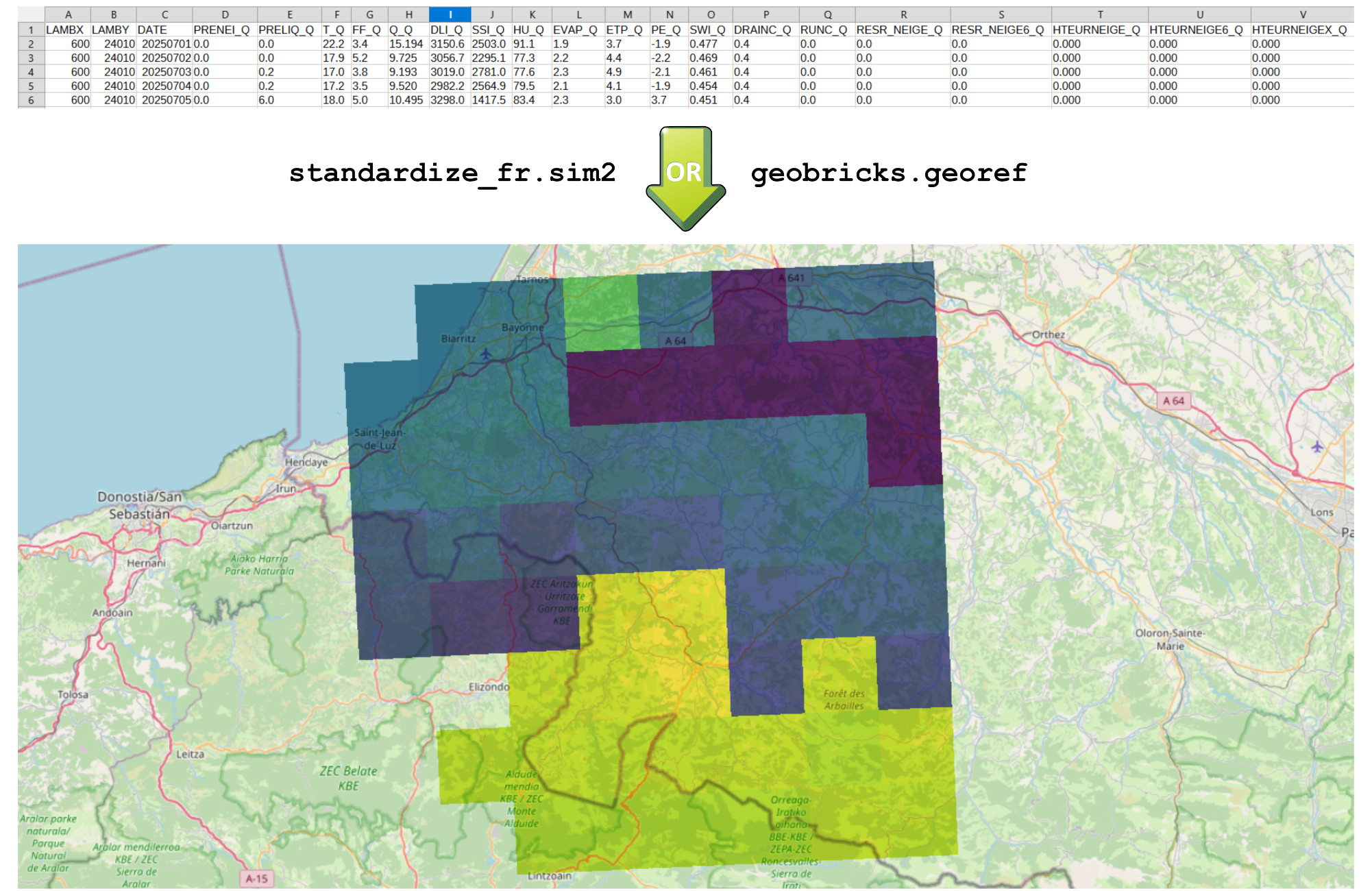
Illustration of standardize_fr.sim2()#
Standardize functions, as well as geobricks.georef(), converts data into geospatial formats easy to view and handle.
Format data#
Once our data have been standardized, they are ready to be formated for our specific application (here CWatM model).
Luckily fos us, CWatM scripts have already been developped in GEOP4TH, so we can easily use them to format our standardized data into inputs for CWatM:
formated_ds = cwatm.meteo(
   ds_clean,
   # optional arguments:
   mask = r"<path/to/your/mask>",
   resolution = <res in meters>,
   ...)
If no script already exist for the application you want to use, you can develop them easily thanks to the geobricks toolbox (as presente below in Generic toolbox).
And most important if you do so… please share them as a GEOP4TH script! 💚 (see Contributor’s guide)
Download datasets#
GEOP4TH intends to include functions to automatically download some common datasets. These functions are based on API whenever available, and aim at simplifying the requests. You will need to import these modules:
from geop4th import (
   download_fr as dl,
   standardize_fr as stz,
)
So far, three French datasets have been implemented in the download_fr module:
as well as one global dataset in the download_wl module:
download_wl.ERA5LandDownloader
Hydrological data over France#
If you are interested in hydrological data over France, the functions download_fr.bnpe() and download_fr.hydrometry() will allow you to
retrieve water withdrawals and river discharges data, based on the Hub’eau API. Compared to this API, the GEOP4TH
functions offer additional ergonomy:
posibility to retrieve data over an area defined with a
mask(also, you are informed if the mask is too large for the request)automatically handle the request page size limit
automatically retrieve both measures and site metadata
For instance:
# To download water withdrawal data ('BNPE') over the last ten available years
dl.bnpe(
   dst_folder = r"<destination/folder/on/your/PC>",
   masks = r"<path/to/your/mask>",
   # (or) departments = <code INSEE>,
   # (or) communes = <code INSEE>,
   start_year = 2012,
   end_year = 2022)
This function will download a collection of files (one per year) as well as the site informations.
Note
These files can then be combined and standardized into one single global file with the
function standardize_fr.bnpe():
stzfr.bnpe(r"<path/to/your/folder/where/files/have/been/downloaded>")
Water withdrawals data#
# To download daily discharge data ('QmnJ') over the last 25 years
dl.hydrometry(
   dst_folder = r"<destination/folder/on/your/PC>",
   masks = r"<path/to/your/mask>",
   start_year = 2000,
   end_year = 2025,
   quantities = 'QmnJ')
This function will download a collection of files (one per year and per station) as well as the station information.
Note
These files can
then be combined and standardized into one single global file with the function standardize_fr.hydrometry():
stzfr.hydrometry(r"<path/to/your/folder/where/files/have/been/downloaded>")
Also note that the standardize functions can also be called through the by_name “portal”, which enables more flexibility in the use of keywords:
stzfr.hydrometry(data)
# is equivalent to
stzfr.by_name(data, 'hydrometry')
#           or      'hydrométrie' (with or without accents)
#           or      'discharge'
#           or      'débit' (with or without spaces, capital letters...)
Generic toolbox#
To develop your own workflows, or simply to use generic geospatial functions, you need first to import the main GEOP4TH toolbox, named geobricks:
from geop4th import (
   geobricks as geo,
)
This geobricks module includes all the elementary generic processing functions. See the API reference page for complete information on the functions.
Open a data file#
The first step would usually be to load a data file.
ds = geo.load_any(<r"path/to/your/file">)
Hint
The r character before the string indicates it is a “raw-string”. This prevents issues with '/' or '\' characters.
The geobricks.load_any() function is designed to load any file into a Python variable. Current supported formats are:
vector data
GeoPackage (.gpkg)
shapefile (.shp)
GeoJSON (.json)
raster data
ASCII (.asc)
GeoTIFF (.tif)
both
netCDF (.nc)
others
CSV (.csv)
JSON (.json)
TIFF (.tif)
To standardize the next operations that you will make on this dataset (data_ds), GEOP4TH loads all previous file formats into
4 types of variables:
all vector data will be loaded as a geopandas.GeoDataFrame
all raster data and netCDF will be loaded as a xarray.Dataset
other data will be loaded either as a pandas.DataFrame (CSV and JSON) or as a numpy.array (TIFF).
Attention
GEOP4TH does not currently support Lidar and point cloud data.
Open an example datafile#
If you do not have any dataset nearby you can also load an example from GEOP4TH:
>>> geo.example('mask')
                                            geometry
0  MULTIPOLYGON (((320145.141 6279295.859, 322407...
>>> geo.example('point')
          time   volume           usage       origin                   geometry
0   2022-12-31   7200.0  DRINKING WATER  groundwater   POINT (-0.8363 42.99877)
1   2018-12-31   9503.0  DRINKING WATER  groundwater   POINT (-0.8363 42.99877)
2   2019-12-31   4497.0  DRINKING WATER  groundwater   POINT (-0.8363 42.99877)
3   2020-12-31   2600.0  DRINKING WATER  groundwater   POINT (-0.8363 42.99877)
4   2018-12-31  27602.0  DRINKING WATER  groundwater   POINT (-0.8363 42.99877)
..         ...      ...             ...          ...                        ...
963 2021-12-31   2703.0      IRRIGATION      surface  POINT (-1.16711 43.52758)
964 2018-12-31   5576.0      IRRIGATION      surface  POINT (-1.16711 43.52758)
965 2020-12-31   2690.0      IRRIGATION      surface  POINT (-1.16711 43.52758)
966 2020-12-31   5967.0      IRRIGATION      surface  POINT (-1.16711 43.52758)
967 2019-12-31   6116.0      IRRIGATION      surface  POINT (-1.16711 43.52758)
[968 rows x 5 columns]
>>> geo.example('tif')
<xarray.Dataset> Size: 64kB
Dimensions:    (x: 125, y: 124)
Coordinates:
  * x          (x) float64 1kB 2.445e+05 2.455e+05 ... 3.675e+05 3.685e+05
  * y          (y) float64 992B 1.882e+06 1.88e+06 ... 1.76e+06 1.758e+06
Data variables:
    band_data  (y, x) float32 62kB nan nan nan nan nan ... nan nan nan nan nan
>>> geo.example('netcdf')
<xarray.Dataset> Size: 540kB
Dimensions:      (x: 11, y: 10, time: 608)
Coordinates:
  * x            (x) float64 88B 2.68e+05 2.76e+05 2.84e+05 ... 3.4e+05 3.48e+05
  * y            (y) float64 80B 1.849e+06 1.841e+06 ... 1.785e+06 1.777e+06
  * time         (time) datetime64[ns] 5kB 2024-01-01 2024-01-02 ... 2025-08-30
    spatial_ref  int64 8B 0
Data variables:
    EVAP_Q       (time, y, x) float64 535kB nan nan nan ... 0.0029 0.0029 0.003
Attributes:
    Conventions:  CF-1.12 (under test)
Note
You can also easily download SIM2 meteorological data as a common netCDF example with
download_fr.sim2(), and discharge timeseries as a common vector example with download_fr.hydrometry().
See Download datasets for more insight.
Georeferencing#
Hint
The next sections are in progress
Raw datasets are often not adequally formatted, so that using them or visualizing them on GIS softwares may raise some issues. This is exactly what standardize functions are for (see Standardize data above).
However, if no standardize function is available, you can try as a first attempt the function geobricks.georef() (indeed, most
standardize workflows call this function). If the CRS is not encoded somewhere in the data, you will need to specify it when calling the function:
>>> data_ds = geo.example('faulty')
<xarray.Dataset> Size: 81kB
Dimensions:  (X: 11, Y: 10, DATE: 91)
Coordinates:
  * X        (X) float64 88B 2.68e+05 2.76e+05 2.84e+05 ... 3.4e+05 3.48e+05
  * Y        (Y) float64 80B 1.849e+06 1.841e+06 ... 1.785e+06 1.777e+06
  * DATE     (DATE) datetime64[ns] 728B 2024-01-01 2024-01-02 ... 2024-03-31
Data variables:
    EVAP_Q   (DATE, Y, X) float64 80kB nan nan nan nan ... 0.0012 0.0012 0.0011
>>> geo.georef(data_ds, crs = 27572)
Georeferencing data...
Standardizing time dimension...
   _ The variable 'DATE' has been renamed into 'time'
   _ Coordinates Reference System (epsg:27572) included.
   _ Standard attributes added for coordinates x and y
<xarray.Dataset> Size: 81kB
Dimensions:      (x: 11, y: 10, time: 91)
Coordinates:
  * x            (x) float64 88B 2.68e+05 2.76e+05 2.84e+05 ... 3.4e+05 3.48e+05
  * y            (y) float64 80B 1.849e+06 1.841e+06 ... 1.785e+06 1.777e+06
  * time         (time) datetime64[ns] 728B 2024-01-01 2024-01-02 ... 2024-03-31
    spatial_ref  int64 8B 0
Data variables:
    EVAP_Q       (time, y, x) float64 80kB nan nan nan ... 0.0012 0.0012 0.0011
Attributes:
    Conventions:  CF-1.12 (under test)
Extracting / merging#
Geospatial data available on download servers are often organized into files in a different way than the one we need to use them.
Merging data can be done with geobricks.merge_data().
On the contrary, if you want to clip your data to a specific area, you can use the geobricks.clip() function.
Reprojecting / transforming / rasterizing#
One of the most common operation with geospatial data is to reproject them into a desired resolution, system of coordinates, alignment, or bounds.
This can be done with the geobricks.transform() function (also named geobricks.reproject()).
Rasterization can be made directly in these functions (by passing the rasterize = True, main_var_list (optional) and rasterize_mode (optional) arguments),
or you can call the geobricks.rasterize() function (which is a partial function derived from geobricks.transform()).
Note
geobricks.clip() and geobricks.rasterize() are partial functions derived from geobricks.transform(). Clipping and rasterizing operations can
directly be called within geobricks.transform().
Converting units#
Variable and dimension units.
Comparing#
geobricks.compare()
Handling of the resolution difference